Banking and Bank Run

Theory and Examples

Fatih Kansoy

2024-02-08

Table of contents

• What: What just happened March 2023?
• How: Back to Basics
• Why: What went wrong with SVB?
• Lessons from Financial History?
• Which: A Model Explains The Bank Run
• Any question?

What: What just happened March 2023?

What Just Happened?

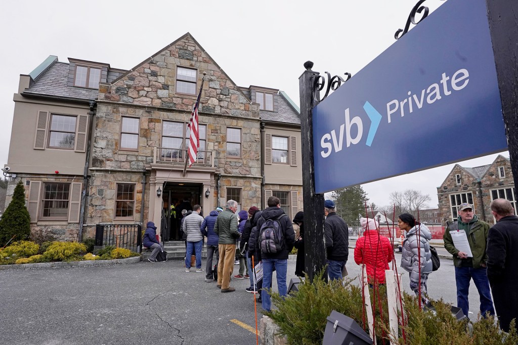
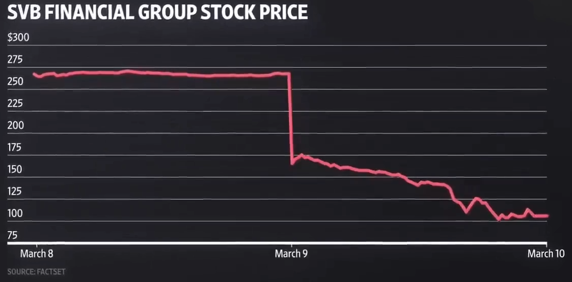
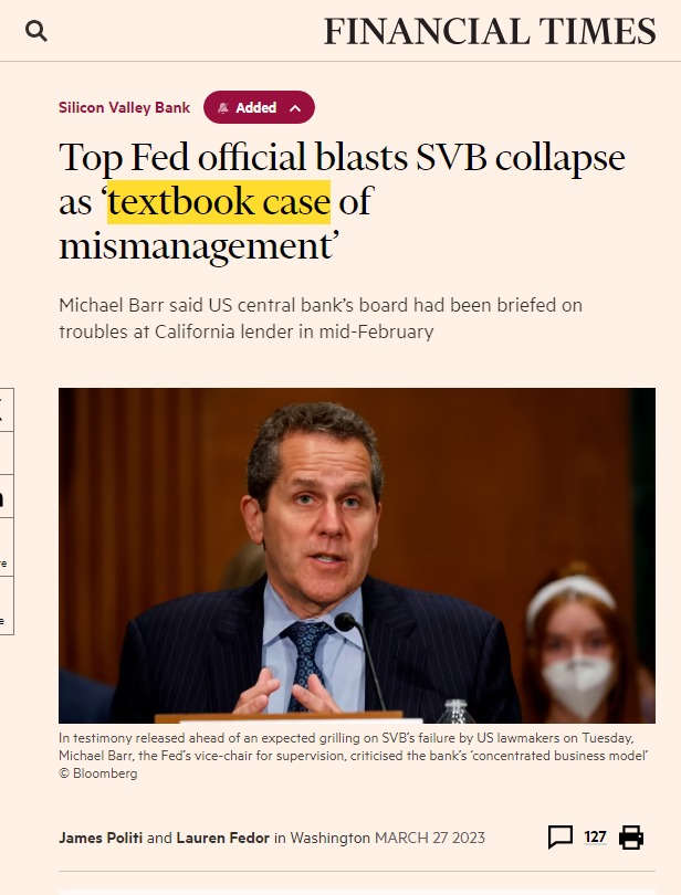
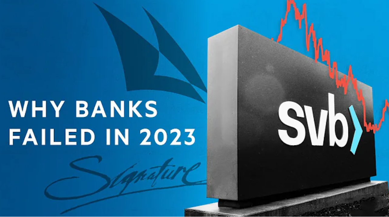
• Friday, March 10 — Silicon Valley Bank (SVB) collapsed and this was the biggest banking collapse in the US since 2008.

• Sunday, March 12 — The FDIC shut down Signature Bank after a run on its deposits by customers who were spooked by the implosion of SVB.

• Wednesday, March 15 — After watching shares in Credit Suisse (CS) collapse by as much as 30%, Swiss authorities announced a backstop for the country’s second-biggest bank.

• Thursday, March 16 — First Republic Bank was teetering on the brink as customers withdrew their deposits. US Treasury and JP Morgan made an agreement to deposit tens of billions of dollars of cash into First Republic to staunch the bleeding. But collappesed May 1 2023.

• Sunday, March 19 — Switzerland’s biggest bank, UBS, agreed to buy its ailing rival Credit Suisse in an emergency rescue deal aimed at stemming financial market panic.

How: Back to Basics

How Banks Work?

Banking Mechanism

No problem in good times

Big problem in rainy days!

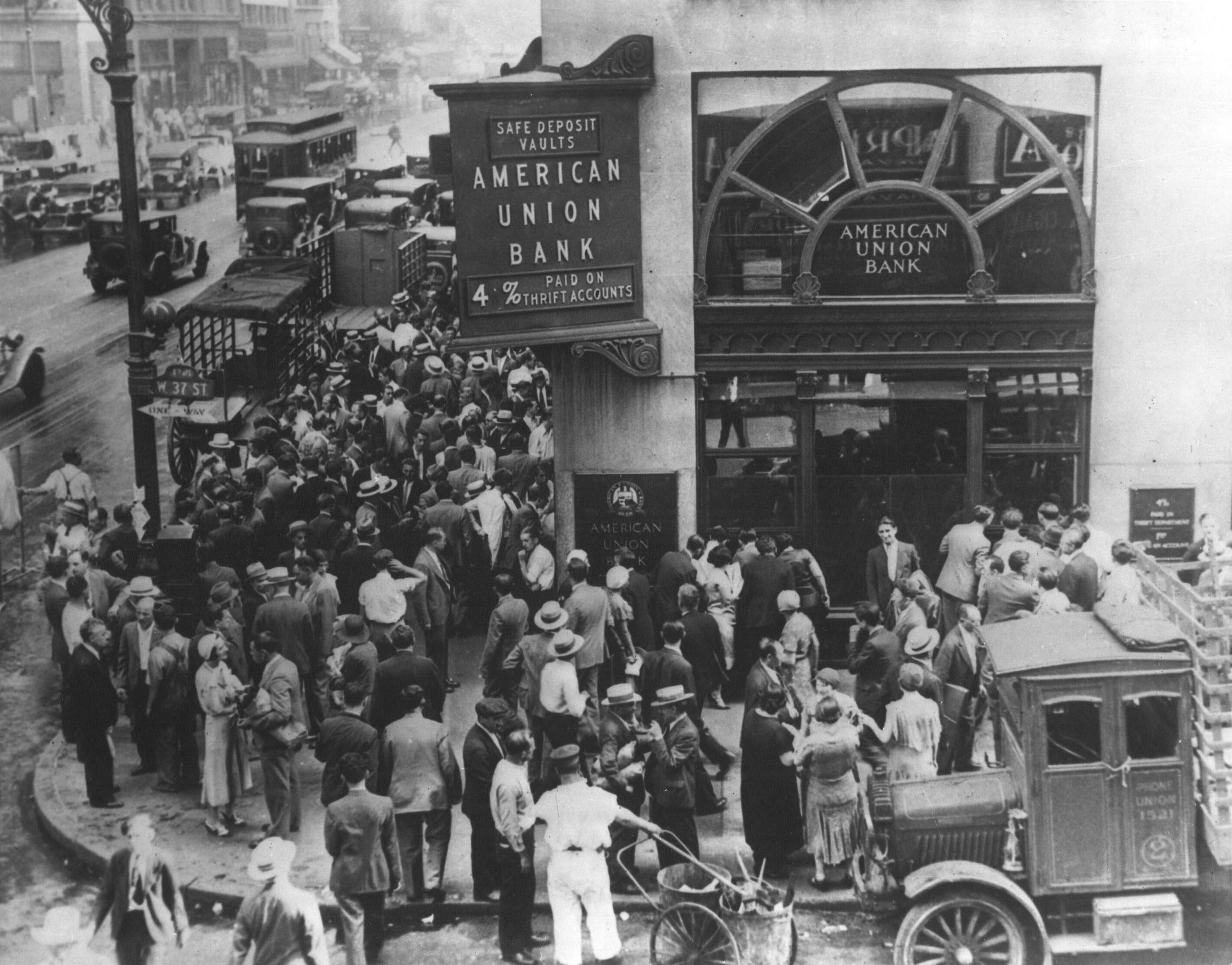
Bank Run in History

Bank Run in Great Depression: April 26, 1932

Power of Bad News

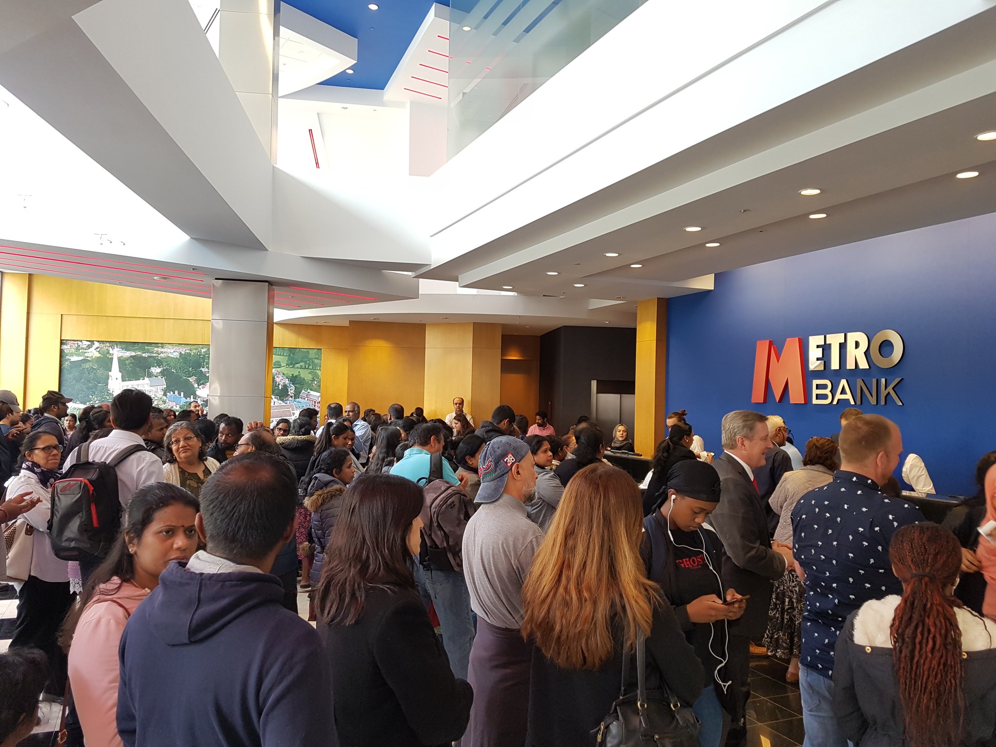
Power of Bad News

The Metro Bank hoax shows the immense power of fake news on WhatsApp

Why: What went wrong with SVB?

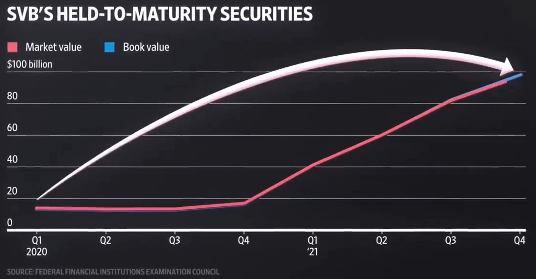
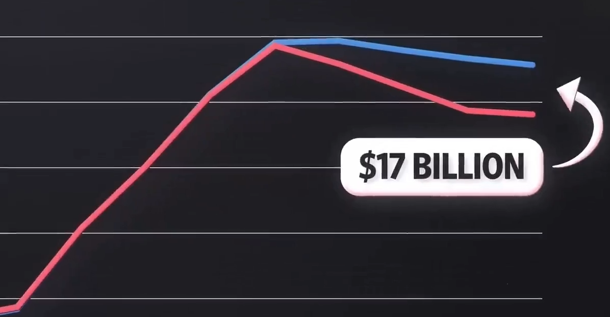
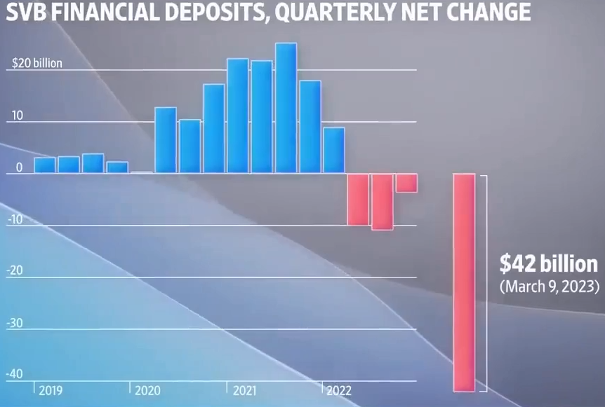
What went wrong with SVB?

• Friday, March 10 — Silicon Valley Bank (SVB) collapsed and this was the biggest banking collapse in the US since 2008.

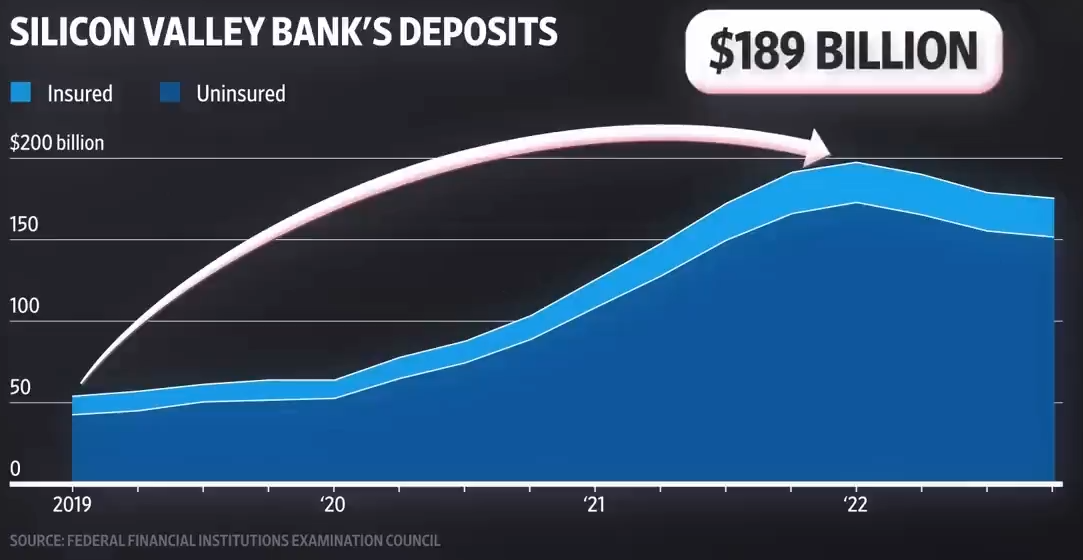
• 2021 The most profitable year ever — 40 years old bank

• 16th Largest Bank —

• Hub of Tech Start-up —

• Roots of the problem –>

The U.S. Federal Funds Rate since 1990

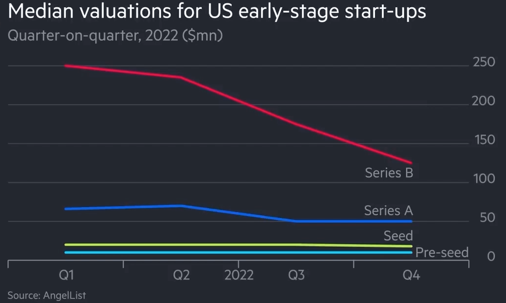
Hub of Tech Companies

The Good Old Days

The Good Old Days

The Good Old Days

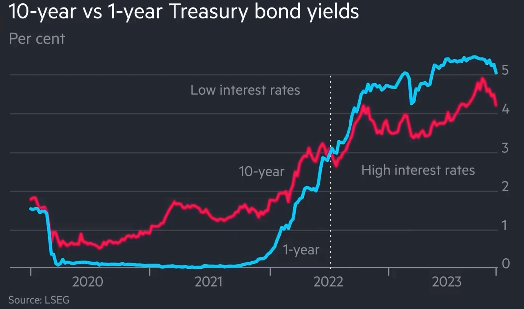
Fed Sent shockwaves

The Good Old Days

The Good Old Days

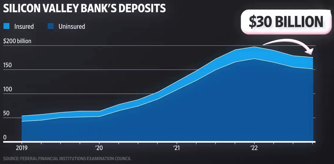
A litle more withdraw

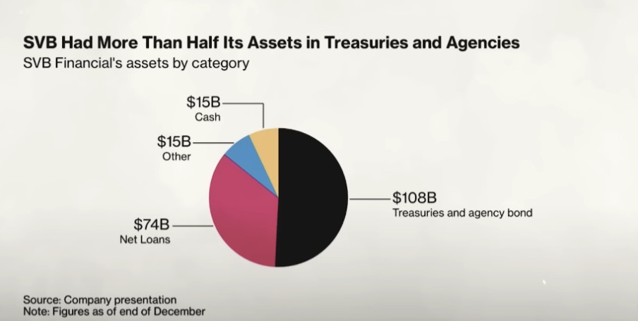
A long-term change

A long-term change

A long-term change

Spark that will set the whole place on fire

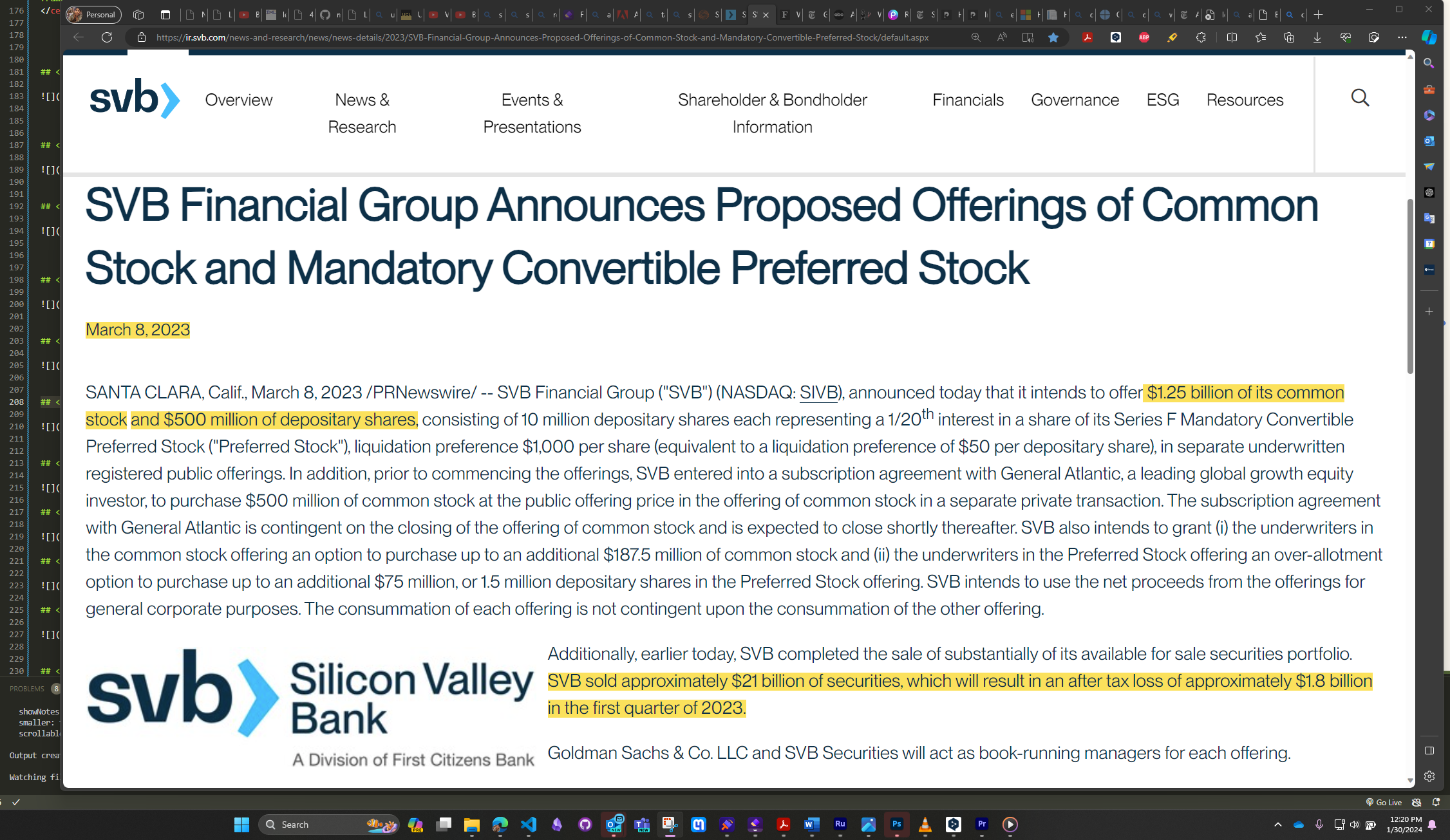
Beginning of the end

The End

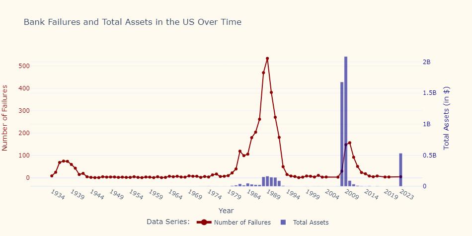
Lessons from Financial History?

Lessons from Financial History?

• Bank Failures
• Source Code

# Working on bank failure. Data from FDIC - Fatih Kansoy
import pandas as pd
import plotly.graph_objs as go
from plotly.subplots import make_subplots

# Load the data
data = pd.read_csv('bankfailure.csv')

# Convert 'FAILDATE' to datetime and extract the year
data['FAILDATE'] = pd.to_datetime(data['FAILDATE'])
data['YEAR'] = data['FAILDATE'].dt.year


# Count unique bank failures per year to ensure no double counting
yearly_failures = data.groupby('YEAR')['ID'].nunique()

# Sum the total assets ('QBFASSET') for each year
yearly_assets = data.groupby('YEAR')['QBFASSET'].sum()

# Generating years from 1934 to 2023, every 5 years, and including 2023
years = list(range(1934, 2024, 5))

# Create subplots with a secondary y-axis
fig = make_subplots(specs=[[{"secondary_y": True}]])

# Add the number of failures plot
fig.add_trace(
    go.Scatter(x=yearly_failures.index, y=yearly_failures, name="Number of Failures", mode='lines+markers', 
               line=dict(color='darkred')),
    secondary_y=False,
)

# Add the total assets plot
fig.add_trace(
    go.Bar(x=yearly_assets.index, y=yearly_assets, name="Total Assets", marker=dict(color='darkblue'), opacity=0.6),
    secondary_y=True,
)

# Update the layout
fig.update_layout(
    title_text='Bank Failures and Total Assets in the US Over Time',
    legend_title_text='Data Series:',
    legend=dict(orientation="h", yanchor="bottom", y=1.02, xanchor="right", x=1),
    paper_bgcolor='#FFF1E0',  # Background color for the entire figure area
    plot_bgcolor='#FFF1E0',
    autosize=True,
    margin=dict(l=50, r=50, b=100, t=100)

)

# Set x-axis and y-axes titles
fig.update_xaxes(title_text="Year", tickvals=years + [2023])

fig.update_yaxes(title_text="Number of Failures", secondary_y=False, color='darkred')
fig.update_yaxes(title_text="Total Assets (in $)", secondary_y=True, color='darkblue')

# Show the figure
fig.show()

Lessons from [Financial] History?

.

Lesson from Financial History?

Regulation \(\neq\) Bureaucracy

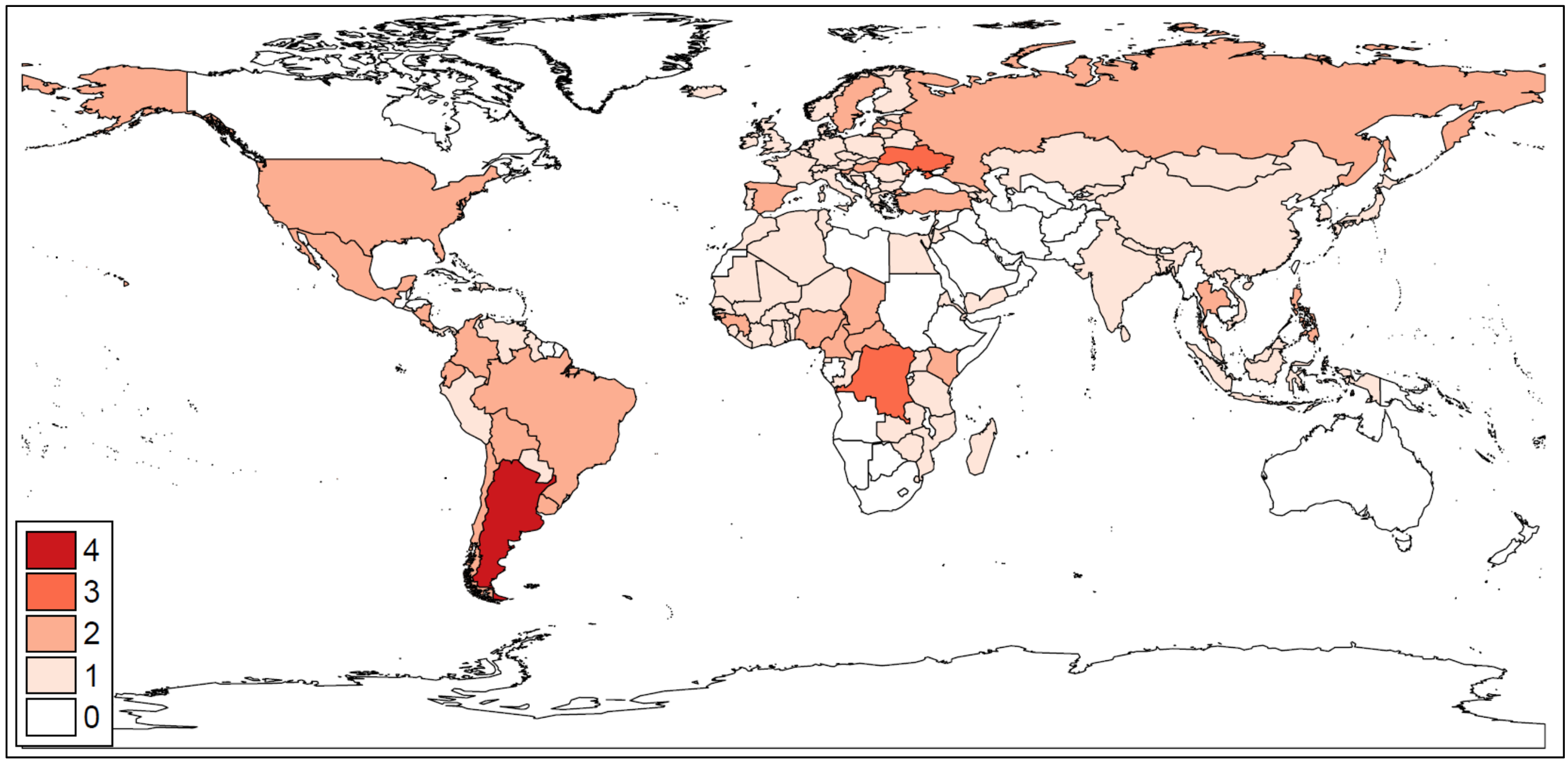
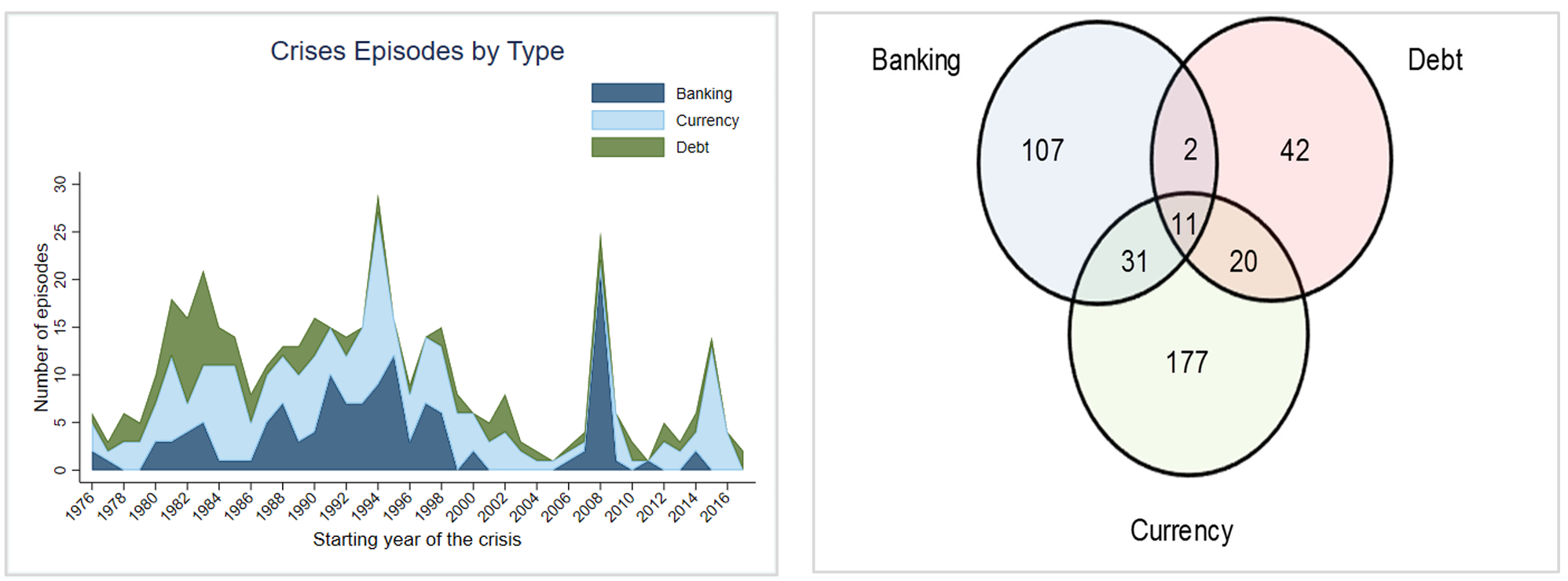
Not Just US and Not Just in 2023

Laeven, M.L. and Valencia, M.F., 2018. Systemic banking crises revisited. IMF.

Not Just the US and Not Just in 2023

Laeven, M.L. and Valencia, M.F., 2018. Systemic banking crises revisited. IMF.

Which: A Model Explains The Bank Run

Models that explain banking

• Diamond & Dybvig (JPE, 1983): Banking Crises & Expectation
• Milgrom & Roberts (Economics, Organization and Management, 1992): Banking Crises & Moral Hazard
• Gertler & Karadi (JME, 2011): Agency Costs and Bank Capital
• Gertler & Kiyotaki (AER, 2015): Combining Financial Accelerator Effects and Bank Runs

Setting:

• Three time periods \(T=0,1,2~\)

• There are many ex ante identical households (investors) 👨👨👨

• One single bank (🏦SVB?)

• Each household ins endowned \(1\) unit of homogeneous good to invest in \(T=0\)

• There are two types of household

  • impatient: only likes consumption in \(T=1\)
  • patient: only likes consumption in \(T=2\)

• Fraction \(\pi~\) of household are Type 1

• In period 1, each household learns her type

• Type is a private information

Timeline and Summary

%%{
  init: {
    'theme': 'base',
    'themeVariables': {
      'primaryColor': '#BB2528',
      'primaryTextColor': '#fff',
      'primaryBorderColor': '#7C0000',
      'lineColor': '#F8B229',
      'secondaryColor': '#006100',
      'tertiaryColor': '#fff',
      'tertiaryBorderColor': '#000' 
    }
  }
}%%
graph LR
    A[Deposit/Investment] -->  X[Decision: Comsume or Wait]  --> Y[Get reward or Lost everything]
    B("-1") -->|Impatient| G(1)
    B --> C(0)
    C ==>|Patient| F(R > 1)
    subgraph "Time=0"
        B
    end
    subgraph "Time=2"
        F
    end
    subgraph "Time=1"
        C
        G
    end

• Denote type \(i\) ’s period- \(T\) consumption by \(C_T^i\)
• Competitive allocation is

\[ \begin{aligned} & C_1^1=1, \quad \quad \quad C_2^1=0 \\ & C_1^2=0, \quad \quad \quad C_2^2=R \end{aligned} \]

Maximisation Problem

• This implies state dependent utility function (with the state private information) \[ U\left(C_1, C_2\right)= \begin{cases}u\left(C_1\right) & \text { if consumer is type } 1 \\ \rho u\left(C_1+C_2\right) & \text { if consumer is type } 2\end{cases} \quad \quad \quad \quad (1) \] with \(R^{-1}<\rho \leq 1\)

• \(u(\cdot)~\) satisfies standard assumptions.

• The contract satisfies: \[ \begin{aligned} c_2^{1 *}=c_1^{2 *}=0 \quad \quad \quad \quad (2) \\ u^{\prime}\left(c_1^{1 *}\right)=\rho u^{\prime}\left(c_2^{2 *}\right) R \quad \quad \quad \quad (3) \\ \pi c_1^{1 *}+(1-\pi) \frac{1}{R} c_2^{2 *}=1 \quad \quad \quad \quad (4) \end{aligned} \]

Investment Strategies:

Short-term investment: Liquid

• Can be terminated in either period 1 or period 2 and yields no return

Long-term investment: - Illiquid

• Investment should be terminated in period 2 and return is \(R>1\)
• Long-term alternative provides a positive return at the cost of being illiquid
• Investment can be terminated in period 1 but it is costly to do so
• Premature termination will yield only the liquidation value \(L<1\)

Altruistic deposit contract

• Bank offers an altruistic deposit contract
• The value \(0 \leq I \leq 1~~\) will be invested in the long term project.

Optimal Allocation

Budget constraints:

• Reflux from the short-term investment \((1-I)~\) has to be high enough to finance \(C_1~~\) that will occur with probability \(\pi\)
  • Period 1: \(\pi \cdot C_1=(1-I)\)
• Reflux from the long-term investment \((I)~\) needs to be high enough to finance \(C_1~~\) that will occur with probability \(\left(1-\pi \right)~\)
  • Period 2: \(\left(1-\pi \right) \cdot C_2=R \cdot I\)

Bank Runs in the Diamond/Dybvig (1983) World

One economy in the Diamond/Dybvig world is characterized by the following parameters: \[ \rho= 0.8, \quad R=1.5, \quad L=0.6, \quad \pi=0.5 \]

The function for the expected utility is given by \[ U=\pi \sqrt{C_1}+\rho\left(1-\pi\right) \sqrt{C_2} \]

• Compute the optimal level of investment (\(I\))
• In the end, we assume that the economy consists out of 100 households.

The Utility and the Budget Constraints

\[ U=\pi \sqrt{\color{red}{C_1}}+\rho\left(1-\pi\right) \sqrt{C_2} \]

Under consideration of the two budget constraints \[ \begin{aligned} \pi C_1 & =1-I \\ \left(1-\pi\right) C_2 & =R \cdot I \end{aligned} \] we can insert \(\color{red}{C_1=(1-I) / \pi}~~~\) and \(~C_2=R \cdot I /\left(1-\pi\right)~~~\) in the utility function: \[ U=\pi \sqrt{\color{red}{\frac{1-I}{\pi}}}+\rho(1-\pi)\sqrt{\frac{R \cdot I}{1-\pi}} \]

• Optimal Investment - Short Cut
• Step-by-step solution

\[ U=\pi \sqrt{\frac{1-\color{red}{I}}{\pi}}+\rho(1-\pi)\sqrt{\frac{R \cdot \color{red}{I}}{1-\pi}} \]

Taking the differential with respect to \(\color{red}{I}\) yields:

\[ \begin{aligned} \frac{d U}{d I} & = \pi \cdot 0.5\left(-\frac{1}{\pi}\right)\left(\frac{1-I}{\pi}\right)^{-0.5} \\ & +\rho\left(1-\pi\right) \cdot 0.5\left(\frac{R \cdot I}{1-\pi}\right)^{-0.5} \cdot \frac{R}{1-\pi}=0 \end{aligned} \]

\[ I=\frac{1}{\frac{\pi}{\rho^2 R\left(1-\pi\right)}+1} \]

\[ \color{red}{I} \approx 0.5 \]

\[ U=\pi\left(\frac{1-I}{\pi}\right)^{0.5}+\rho\left(1-\pi\right)\left(\frac{R \cdot l}{1-\pi}\right)^{0.5} \]

Taking the differential with respect to (I) yields:

\[ \begin{aligned} \frac{d U}{d I} & = \pi \cdot 0.5\left(-\frac{1}{\pi}\right)\left(\frac{1-I}{\pi}\right)^{-0.5} \\ & +\rho\left(1-\pi\right) \cdot 0.5\left(\frac{R \cdot I}{1-\pi}\right)^{-0.5} \cdot \frac{R}{1-\pi}=0 \end{aligned} \]

Putting (I) on the RHS and afterwards out of brackets yields:

\[ \begin{gathered} 1=I\left(\frac{R \pi}{\rho^2 R^2\left(1-\pi\right)}+1\right) \\ I=\frac{1}{\frac{R \pi}{\rho^2 R^2\left(1-\pi\right)}+1} \\ I=\frac{1}{\frac{\pi}{\rho^2 R\left(1-\pi\right)}+1} \end{gathered} \]

Since in our numerical example \(\pi=1-\pi\), the probabilities will disappear. With \(\rho=(2 / 3)^{0.5}\) and \(R=3/2\), we get:

\[ I=\frac{1}{\frac{1}{\rho^2 R}+1}=\frac{1}{\frac{1}{\left[\left(\frac{2}{3}\right)^{0.5}\right]^2 \cdot \frac{3}{2}}+1}=\frac{1}{\frac{1}{\frac{2}{3} \cdot \frac{3}{2}}+1}=\frac{1}{1+1}=0.5 \]

Numerical solution

• 100 households \(\Rightarrow 100~~\) goods
• Bank invest 50 goods at interest rate of \(R=1.5\).
• This will lead to 75 goods in period 2 .

On average,

• 50 customers of type 2 will show up at the bank in period 2, so that each type 2 household can consume \(C_2=\frac{75}{50}=1.5\)

• 50 goods are invested in the non-interest bearing asset.

• On average 50 type 1 households will show up in period 1. Thus \(C_1=\frac{50}{50}=1 ~~\) goods.

• \(C_1=1~~\) and \(C_2=1.5\)

• If type 2 households believe that the banking system is stable: Since \(C_2>C_1~~\), type 2 households have no incentive to queue up already in period 1 !

What Just Happened?

• Period 1: \(\pi \cdot C_1=(1-I)\)
• Period 2: \(\left(1-\pi \right) \cdot C_2=R \cdot I\)
• Terminated in period 2 \(R>1\)
• Premature termination \(L<1\)

%%{
  init: {
    'theme': 'base',
    'themeVariables': {
      'primaryColor': '#BB2528',
      'primaryTextColor': '#fff',
      'primaryBorderColor': '#7C0000',
      'lineColor': '#F8B229',
      'secondaryColor': '#006100',
      'tertiaryColor': '#fff',
      'tertiaryBorderColor': '#000' 
    }
  }
}%%
graph LR
    
    B("-1") -->|Impatient| G(1)
    B --> C(0)
    C ==>|Patient| F(R > 1)
    subgraph "Time=0"
        B
    end
    subgraph "Time=2"
        F
    end
    subgraph "Time=1"
        C
        G
    end

What Just Happened?

• Period 1: \(\pi \cdot C_1=(1-I)\)
• Period 2: \(\left(1-\pi \right) \cdot C_2=R \cdot I\)
• Terminated in period 2 \(R>1\)
• Premature termination \(L<1\)

%%{
  init: {
    'theme': 'base',
    'themeVariables': {
      'primaryColor': '#BB2528',
      'primaryTextColor': '#fff',
      'primaryBorderColor': '#7C0000',
      'lineColor': '#F8B229',
      'secondaryColor': '#006100',
      'tertiaryColor': '#fff',
      'tertiaryBorderColor': '#000' 
    }
  }
}%%
graph LR
    
    B("-1") -->|Impatient| G(1)
    B --> C(0)
    C ==>|Patient| F(R > 1)
    subgraph "Time=0"
        B
    end
    subgraph "Time=2"
        F
    end
    subgraph "Time=1"
        C
        G
    end

• The bank liquidates the long term investment of \(I=50~~\) at \(L=0.6~~~\)
• Which yields \(I \cdot L=50 \cdot 0.6=30~~~~\) goods.
• Hence, the bank can distribute \(50+30=80~~~\) goods in period 1 .
• This last only for \(80 \div 1.0=80~~~\) customers.
• 20 customers loose their wealth completely.
• If you panic, panic early!

Main Ideas of Diamond-Dybvig

• Liquidity Transformation: Banks transform liquid deposits into illiquid loans, providing liquidity to depositors who may need their funds back on short notice while investing in longer-term projects that cannot be quickly liquidated without loss.

• Sequential Service Constraint: The model assumes that banks operate on a first-come, first-served basis. This creates a situation where, if all depositors try to withdraw their funds simultaneously (fearing that the bank will run out of liquid assets), the bank will indeed run out of cash, leading to a self-fulfilling prophecy.

• Multiple Equilibria: One of the critical insights from the model is the existence of multiple equilibria: one where everyone trusts the bank and does not rush to withdraw (a stable equilibrium), and another where a panic leads to a bank run (an unstable equilibrium).

• Role of Expectations: The possibility of a bank run is driven largely by depositors’ expectations. If depositors expect others to withdraw their money, they have an incentive to withdraw theirs as well, leading to a bank run

Implications and Solutions

• Lender of Last Resort: By providing liquidity to banks facing runs, the lender of last resort can prevent the temporary liquidity problem from becoming a solvency crisis, stabilizing the banking system.

• Deposit Insurance: This reduces the incentive for depositors to withdraw their money in a panic, thereby preventing bank runs.

• Moral Hazard: Deposit insurance and lender of last resort facilities can also introduce moral hazard. Banks might take on riskier investments knowing they’re insured or that they can be bailed out, potentially leading to more significant problems in the long run.

• Inherent Risk in Banking System: Model highlights the inherent risk in the banking system due to liquidity mismatch and the reliance on short-term deposits to fund long-term investments. This structural vulnerability necessitates regulatory oversight, prudential regulation, and safety nets like deposit insurance and central bank interventions to maintain stability and confidence in the financial system.

Any question?

Thank you!